Introduction
DISCLAIMER
The tutorial below is for metaSNV v1.
For metaSNV v2, please see the updated manual and the GitHub page.
This tutorial reproduces the analysis presented in the forthcoming manuscript. The data associated with the study is publicly available, and the method behind the computational procedures is explained in the article. Here, we present a detailed tutorial to reproduce our work in the article using metaSNV.
Installation & compilation
Download statically compiled release version here or clone metaSNV from the gitlab repository and follow the instructions in the readme to install and compile the pipline package. MetaSNV is mainly written in c++ and python, and licensed under the terms of the GNU General Public License (GPL). Setup and compile the pipeline, download the reference database and integrate the metaSNV installation into your linux environment.
Dependencies
Installation
Installing dependencies on Ubuntu/debian
On an Ubuntu/debian system, the following sequence of commands will install all required packages (the first two are only necessary if you have not enabled the universe repository before):
                sudo add-apt-repository "deb http://archive.ubuntu.com/ubuntu $(lsb_release -sc) universe"


                sudo apt-get update

                sudo apt-get install libhts-dev libboost-dev
Installing dependencies using anaconda
If you use anaconda, you can create an environment with all necessary dependencies using the following commands:
                conda create --name metaSNV boost htslib pkg-config

                source activate metaSNV

                export CFLAGS=-I$CONDA_ENV_PATH/include

                export LD_LIBRARY_PATH=\$CONDA_ENV_PATH/lib:$LD_LIBRARY_PATH
If you do not have a C++ compiler, anaconda can also install G++:
                conda create --name metaSNV boost htslib pkg-config

                source activate metaSNV


                # Add this command:

                conda install gcc


                export CFLAGS=-I$CONDA_ENV_PATH/include

                export LD_LIBRARY_PATH=\$CONDA_ENV_PATH/lib:\$LD_LIBRARY_PATH
Compilation
make
If make does not work, edit the file `SETUPFILE` to contain the correct paths to Boost and htslib.
Environment variables
Make metaSNV quickly accessible by running these commands in your current shell session or include them permanently into your bashrc. Throughout this tutorial we assume that metaSNV is in your $PATH variable:
                    export PATH=/path/2/metaSNV:$PATH

                    export PATH=/path/2/python:$PATH

                    export PATH=/path/2/samtools:$PATH
Note: Replace '/path/2' with the respective global path.
Reference & Samples
Reference
To download the reference database, run the getRefDB.sh in the parent directory of your metaSNV installation or download the archive including the reference genomes, gene annotations and the genome definitions file here. The script will prompt you to select one of the two available references and to confirm the download. The reference databases freeze9 and freeze11 represent 1753 and 5278 species respectively. To reproduce the analysis in the paper, select freeze9.
./getRefDB.sh
The script downloads the database into a new folder (db/).
Note: It is also possible to set up your custom database, a multi-sequence file in FASTA format.
Samples
The dataset used in the article is a subset of the Human Microbiome Project (HMP) samples which are freely available online. For the sake of a quick illustration of metaSNV's basic workflow you can simply run the getSamplesScript.sh in the EXAMPLE folder of your metaSNV installation to download a small dataset of six samples or download the archive here.
                    cd EXAMPLE/

                    ./getSamplesScript.sh
Alignment
MetaSNV does not ship with an aligner to keep it as versatile as possible. It is up to the user to choose the preferred method of choice. Align your metagenomic sequences to your reference of choice before running metaSNV. You can skip this step if you use the provided samples in the example (dataset).
Quality control
For the analyses and benchmarking experiments shown in the paper, the metagenomic DNA sequences were quality controlled (mini-mum read length = 45 bp; minimum base quality score = 20) and filtered for human contaminations using MOCAT (version 1.2) (Kultima et al., 2012). In brief, low-quality reads (option read trim filter with length cutoff 45 and quality cutoff 20) were removed and HQ reads were screened against the Illumina adapter sequences in a custom-made fasta file (option screen fastafile with e-value 0.00001 using USEARCH (Edgar, 2010) version 5). Subsequently, the adapter-screened reads were mapped against the human genome version 19 (option screen with alignment length cutoff 45 and minimum 90 % sequence identity). Reads mapping the human reference genome were discarded.
Alignment
Screened and filtered HQ metagenomic DNA sequences (HQ reads) were aligned to the prokaryotic reference database using the Burrows-Wheeler Alignment tool (BWA) (Li and Durbin, 2009) wrapped into NGLess. Large metagenomic datasets and databases can be easily handeled using NGLess. We used NGLess with these parameters (min_identity_pc=97 and min_match_size=45) for mapping the metagenomes with BWA. Only unique mappers are kept. After installing ngless it is recommended to first index the reference. Due to the sheer size of freeze9 or freeze11 this step will take up to 24 hours.
Here is the NGLess recipe we used:
                    ngless "0.0"
                    import "mocat" version "0.0"

                    import "batch" version "0.0"

                    import "parallel" version "0.0"

                    import "samtools" version "0.0"


                    sample = lock1(readlines('sampleNames.txt'))

                    input = fastq('/rmuench/FASTA/' + sample + '.fq.gz')

                    FREEZE11 = 'db/freeze11.genomes.representatives.fa'


                    mapped = map(input, fafile=FREEZE11, __extra_bwa=['-a'])

                    mapped = select(mapped, keep_if=[{mapped}, {unique}])

                    mapped = select(mapped) using |mread|:

                    mread = mread.filter(min_identity_pc=97, min_match_size=45)

                    mapped = samtools_sort(mapped)

                    write(mapped, ofile='outputs/' + sample + '.Freeze11.sorted.bam')
Note: 'sampleNames.txt' is a file with the sample names, one sample name per line.
Alignment example using BWA
If you decide to use BWA stand alone you can follow these simple steps to align your shotgun sequenced metagenomic reads using BWA. The following example has no biological relevance but demonstrates the basic commands. You can download the fastq files for the six aligned samples in the EXAMPLE as well as a small three genome reference fasta file here: "three-genome-ref" [65 Mb].
First, we index the reference:
$ bwa index three-genome-ref.fa
Subsequently, the fastq files can be aligned and converted to SAM/BAM format:
                    $ bwa aln three-genome-ref.fa s1.fastq  > s1.sai

                    $ bwa samse three-genome-ref.fa s1.sai s1.fastq > s1.sam

                    $ samtools view -b s1.sam > s1.bam

                    $ samtools sort s1.bam > sample1.bam
Once all the samples are aligned you can proceed with the three main processing steps (Data processing).
Note: BAM files need to be sorted!
Data Processing

|
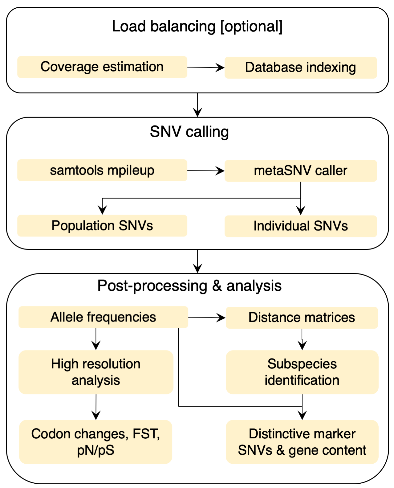
The pipeline input is a list of alignment files in SAM/BAM format, which contains the results of mapping metagenomic samples to a genome reference database. This reference may be a custom one created by the user or the one deployed with the current software, previously described (Mende et al., 2016). Internally, metaSNV is structured as a sequence of three processing steps (Figure left): 1. Determine the average coverage over each reference genome in each sample. 2. Compute the genomic variation and output all of the variant positions that meet the imposed quality criteria. 3. Provide basic analyses of this landscape and allow the user to compute per species pair-wise distance matrices of samples. |
|---|
Workflow
The entire variant calling workflow can be completed with two commands. The command lines can also be printed for advanced usage and runtime optimization using parallel computing (see Advanced usage).
Input files
Required files
'all_samples' = a list of all BAM files, one /path/2/sample.bam per line (no duplicates).
'ref_db' = the reference database in fasta format (f.i. multi-sequence fasta).
'gen_pos' = a list with start and end positions for each sequence in the reference (format: sequence\_id start end).
Optional files
'db_ann' = a gene annotation file for the reference database (format: ).
Post-processing (filtering & analysis)
metaSNV_post.py project_dir [options]
Note: Requires SNV calling to be done!
Output
After successfully running the pipeline you will find the following files and folder in the project directory:Files
'all_samples' = the sample_list used for this project.
'tutorial.all_cov.tab' = average vertical genome coverage for every genome and sample.
'tutorial.all_perc.tab' = horizontal genome coverage (percentage) for every genome and sample.
Folders
'bestsplits/' = index files used for the load balancing step (--threrads or --n_splits).
'cov/' = coverage files after the coverage estimation using qaCompute.
'distances/' = pair-wise distances computed between samples based on the SNV profiles for each species (manhattan, major allele and evolutionary distances).
'filtered/' = discovery sets: filtered SNV profiles for the sample subsets for each species.
'snpCaller/' = contains the raw SNV files, one file per split.
Tutorial
Start in the metaSNV parent directory after downloading the reference database (db/) and the samples (see: reference & samples).Generate the sample list ('all_samples'):
$ find `pwd`/EXAMPLE/samples -name "*.bam" > sample_list
Run the SNV calling step:
$ python metaSNV.py tutorial sample_list db/freeze9.genomes.RepGenomesv9.fna --threads 8
Run filtering and post processing:
$ python metaSNV_post.py tutorial
Note: Try the filtering options if you aligned samples to the three-genome-ref (see below).
Advanced usage
If you want to run a lot of samples and would like to use the power of your cluster, use the --print-commands option which will print out the command lines. You need to run these command lines manually but you can decide on how to schedule and manage them.Coverage estimation
$ python metaSNV.py tutorial sample_list db/freeze9.genomes.RepGenomesv9.fna --n_splits 8 --print-commands
Note the addition of the "--print-commnads". This will print out one-liners that you need to run. When done, you need to run the same command again for the actual SNV calling (see next section).
Variant calling
$ python metaSNV.py tutorial sample_list db/freeze9.genomes.RepGenomesv9.fna --n_splits 8 --print-commands
Note: This will calculate the "load balancing" and give you the commands for running the SNV calling.
Post-Processing
Taxon, sample and position filters are applied post SNP calling. Specifically, we require that a genome has a horizontal coverage of 40% or higher and a vertical coverage of at least 5x (default). Both these cut-offs can be customized by the user, though we recommend using the proposed ones to ensure the accuracy of the distances estimation. For downstream processing, pair-wise distance matrices are also computed between all samples.
Filtering & distance computation:
./metaSNV_post.py tutorial/ -b 2.0 -d 1.0 -m2 -c 2 -p 0.04
metaSNV_post.py helps you to filter the 'raw' output in the 'tutorial/snpCaller/' subdirectory. The script computes the SNV allele frequencies and pair-wise distances between samples based on these SNV profiles for each species. Read the help message (-h) to get familiar with the script. For the purpose of demonstration, we used all the possible options and set the following filters: Species filter (-m 2, minimum of two samples per species), sample filters (-b 2.0, genome coverage breads [percentage of reference genome covered at least 1 X] and -d 1.0, coverage depth [average coverage depth ≥ 1.0 reads]) and position filters (-c 2, least amount of reads per site and -p 0.04, required proportion of samples passing the -c condition at that position)
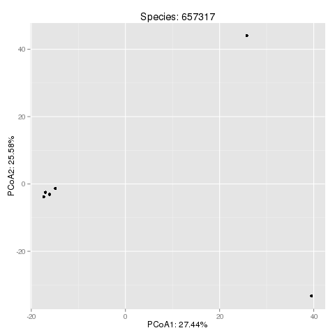
PCoA projection of the SNP space:

This plot is an example output for the Eubacterium rectale (taxonomy id '657317'). You can find further information about the species corresponding to the taxonomy id's at the NCBI Taxonomy Homepage.
